library(tidyverse) # pretty much always...
library(readxl) # for reading excel files
# install.packages("here") # install the package if you haven't yet
library(here) # for using relative file paths4 Data Import
4.1 Learning Objectives
4.2 R for Data Science 2e Chapter
Work through the R for Data Science 2e Chapter
The rest of this chapter assumes you’ve read through R for Data Science (2e) Chapter 7 - Data import, and Chapter 20 - Spreadsheets. Run the code as you read. We highly suggest doing the exercises at the end of each section to make sure you understand the concepts. The rest of this chapter in this textbook will assume this knowledge and build upon it to learn about Sustainable Finance applications.
Spreadsheets:
4.3 Resources
4.3.1 Cheatsheet
Print, download, or bookmark the data import cheatsheet. Spend a few minutes getting to know it. This cheatsheet will save you a lot of time later.
4.3.2 Package Documentation
The readr package website provides extensive documentation of the package’s functions and usage.
Also look at the website for readxl, readr’s close cousin, which we will use in this chapter to read in Excel files.
4.4 Applying Chapter Lessons to Sustainable Finance
Your boss has an interview on Bloomberg TV next week. They want to say something smart about critical minerals and the energy transition. It’s your job to do the research that will make your boss sound smart. She wants charts and key facts by Monday.
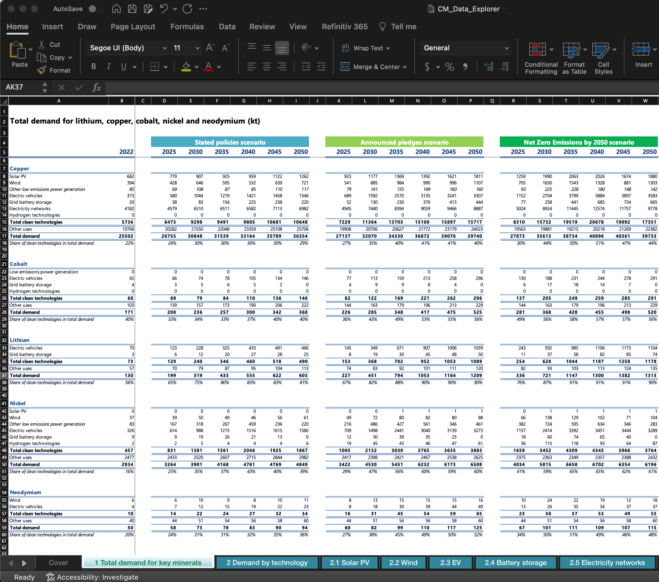
You see that the International Energy Agency (IEA) has an interesting recent report on critical minerals, and an accompanying dataset. The dataset has an excellent table that provides demand estimates for critical minerals based on three policy scenarios.
This is exactly the data you need, but how the heck do you get data formatted like this into R?
This spreadsheet is tricky, but not uncommon. Once you learn how to import and clean a spreadsheet like this, most others you encounter will be much easier.
4.4.1 Data import workflow
Why worry about workflow? New projects are always one-off. And then you find yourself updating the project every year, month, or week for the next three years. Taking a little time up front to keep things organized pays off.
As you become an experienced data analyst, you can come up with your own workflow. For now, here’s a simple start.
Start your new project by creating a new R Studio project.
Create folders called
data-raw, to keep a copy of the raw data, anddatafor your processed data.Create a new Quarto script in
data-raw, where you import and tidy the data. Write the resulting script to thedatafolder. In all future sessions, you’ll be able to skip straight to the fun stuff (making sense of your data), and just read the cleaned data from thedatafolder.
When you need to update your analysis, or use this data in another project, you’ll thank yourself.
4.4.2 Messy Excel Tables
Data saved in excel spreadsheets is generally formatted for humans, not for machines.
The IEA workbook we want to read is formatted like a table in a report. It’s good for eyeballing figures. Download the spreadsheet from the IEA, and spend a few minutes trying to figure out the biggest takeaways.
But you get paid the big bucks to do cool work because you have data analysis power tools to extract non-obvious insights from the data. That’s why they hired you.
So, how do we import and tidy this data so we can start using our tidyverse toolkit?
First, let’s take stock of the challenges we’ll face:
Untidy Wide Data: The data is presented in wide format, with the years as column headers. This is common, as we saw in the last chapter.
Multi-Row Column Headers: The column headers are two rows. First, in row 4, there are three policy scenarios. In the next row, there are six years of projections.
15 Mini Tables: There are five Critical Minerals listed in the rows. In essence this means there are 15 different smaller tables (3x policy scenarios for 5 Critical Minerals).
Units: The bottom row of each of these sub-tables is in a different unit (percent) compared to the other datapoints (kilotons).
After you import and clean this gnarly excel table, other more simply formatted spreadsheets will be a piece of cake.
4.4.3 Getting Started
4.4.3.1 Setup:
R Studio Project: If you’re not already working inside an R Studio Project, create one.
Create folders: Create one folder inside your project called
data-rawand another calleddata.Download Spreadsheet: Download the Critical Minerals Demand Dataset Excel spreadsheet from the IEA. If you haven’t done so previously, you’ll have to create a (free) login for the IEA website. The spreadsheet is named
CM_Data_Explorer.xlsx. Save it to thedata-rawfolder you just created.
4.4.4 Work Hard To Be Lazy
Good data analysts work hard to be lazy.
Functions are a superpower for data analysts. We will create code to import the data for one of the minerals. Then we’ll make a function out of that code, and we’ll be able to import the data for the four other minerals with just a few lines of code.
4.4.4.1 Creating a function to read in our worksheet
We will be reading in this spreadsheet in multiple sections. Copying and pasting our code is annoying and prone to error. We’ll create a function that enables us to read our worksheet simply by providing the cell ranges.
First, we are going to use here::here() to create relative file paths. You can read more about here here. For now, know that it will save you time and anguish by allowing you to painlessly create file paths relative to your project’s main folder. Here, we provide it with the folder name, data-raw, and the file name CM_Data_Explorer.xlsx, and it creates the absolute file path on your computer, which will be different than mine.
path_to_sheet <- here("data-raw", "CM_Data_Explorer.xlsx")

path_to_sheet
[1] "/Users/teal_emery/Dropbox/DataScience/sais_susfin_textbook/data-raw/CM_Data_Explorer.xlsx"We’re going to be reading this table in multiple chunks. To avoid repeating code over and over, we’ll use purrr::partial() to create a custom function that pre-populates most of the inputs in readxl::read_excel()
read_key_minerals_sheet <- partial(
  # provide the function, in this case readxl::read_excel()
  .f = read_excel,
  # provide any arguments you want filled in
  path = path_to_sheet,
  sheet = "1 Total demand for key minerals",
  col_names = FALSE
)

# now all we have to do is provide the range
sheet_header <- read_key_minerals_sheet(range = "A4:W5")

sheet_header
# A tibble: 2 × 23
...1 ...2 ...3 ...4 ...5 ...6 ...7 ...8 ...9 ...10 ...11 ...12 ...13
<lgl> <dbl> <lgl> <chr> <dbl> <dbl> <dbl> <dbl> <dbl> <lgl> <chr> <dbl> <dbl>
1 NA NA NA State… NA NA NA NA NA NA Anno… NA NA
2 NA 2022 NA 2025 2030 2035 2040 2045 2050 NA 2025 2030 2035
# ℹ 10 more variables: ...14 <dbl>, ...15 <dbl>, ...16 <dbl>, ...17 <lgl>,
# ...18 <chr>, ...19 <dbl>, ...20 <dbl>, ...21 <dbl>, ...22 <dbl>,
# ...23 <dbl>4.4.4.2 Tidying the headers
We are going to turn these into tidy columns using a few steps:
Transpose the data from two rows into two columns using
t().Turn it back into a
tibbleobject.t()turned it into adata.frame.Give meaningful column names
fill()down the scenario namesThe top portion still remains
NAvalues, replace those with “Current Year”
sheet_header_processed <- sheet_header |>
  # transpose the data
  t() |>
  # turn it back into a tibble
  as_tibble() |>
  # make them meaningful
  rename(scenario = V1, year = V2) |>
  # fill scenario down
  fill(scenario) |>
  #insert "Current" at top
  replace_na(list(scenario = "Current Year"))

sheet_header_processed
# A tibble: 23 × 2
scenario year
<chr> <chr>
1 Current Year <NA>
2 Current Year 2022
3 Current Year <NA>
4 Stated policies scenario 2025
5 Stated policies scenario 2030
6 Stated policies scenario 2035
7 Stated policies scenario 2040
8 Stated policies scenario 2045
9 Stated policies scenario 2050
10 Stated policies scenario <NA>
# ℹ 13 more rowsLet’s review what we have now. We have a tibble with two variables: scenario, and year. There are 23 rows (observations). The rows where year is NA are the columns that were left empty for spacing in the Excel table. We’ll deal with those later. Now that this is in a tidy format, you can filter or group by year or by policy scenario, which will be helpful when analyzing the data.
4.4.4.3 Get The Mineral Name
We’ll want to create a column that has the mineral name. We can get this by reading in the cell where the name of the mineral is written in the spreadsheet using our read_key_minerals_sheet() custom function.
mineral_name <- read_key_minerals_sheet(range = "A7") |>
  pull()

mineral_name
[1] "Copper"4.4.4.4 Get The Table
Next we read in the Copper table.
mineral_info <- read_key_minerals_sheet(range = "A8:W18")

mineral_info
# A tibble: 11 × 23
...1 ...2 ...3 ...4 ...5 ...6 ...7 ...8 ...9 ...10
<chr> <dbl> <lgl> <dbl> <dbl> <dbl> <dbl> <dbl> <dbl> <lgl>
1 Solar PV 6.82e+2 NA 7.79e+2 9.07e+2 9.25e+2 9.59e+2 1.12e+3 1.26e+3 NA
2 Wind 3.94e+2 NA 4.28e+2 6.46e+2 5.95e+2 5.32e+2 6.39e+2 7.21e+2 NA
3 Other lo… 8.50e+1 NA 6.90e+1 1.08e+2 8.69e+1 8.47e+1 1.10e+2 1.17e+2 NA
4 Electric… 3.73e+2 NA 5.80e+2 1.04e+3 1.22e+3 1.42e+3 1.46e+3 1.35e+3 NA
5 Grid bat… 2.04e+1 NA 3.84e+1 8.27e+1 1.54e+2 2.25e+2 2.38e+2 2.20e+2 NA
6 Electric… 4.18e+3 NA 4.58e+3 6.51e+3 6.51e+3 6.58e+3 7.11e+3 6.98e+3 NA
7 Hydrogen… 3.20e-3 NA 3.88e-3 6.76e-3 6.53e-3 6.99e-3 8.90e-3 1.45e-2 NA
8 Total cl… 5.74e+3 NA 6.47e+3 9.30e+3 9.49e+3 9.80e+3 1.07e+4 1.06e+4 NA
9 Other us… 1.98e+4 NA 2.03e+4 2.15e+4 2.20e+4 2.34e+4 2.51e+4 2.57e+4 NA
10 Total de… 2.55e+4 NA 2.68e+4 3.08e+4 3.15e+4 3.32e+4 3.58e+4 3.64e+4 NA
11 Share of… 2.25e-1 NA 2.42e-1 3.01e-1 3.01e-1 2.96e-1 2.98e-1 2.93e-1 NA
# ℹ 13 more variables: ...11 <dbl>, ...12 <dbl>, ...13 <dbl>, ...14 <dbl>,
# ...15 <dbl>, ...16 <dbl>, ...17 <lgl>, ...18 <dbl>, ...19 <dbl>,
# ...20 <dbl>, ...21 <dbl>, ...22 <dbl>, ...23 <dbl>4.4.4.5 Putting It All Together
Get the column names. Because we specified colnames = FALSE as an argument in readxl::read_excel() when creating our read_key_minerals_sheet() the column names are in the format ...1, ...2, etc.
mineral_info_col_names <- names(mineral_info)

mineral_info_col_names
[1] "...1" "...2" "...3" "...4" "...5" "...6" "...7" "...8" "...9"
[10] "...10" "...11" "...12" "...13" "...14" "...15" "...16" "...17" "...18"
[19] "...19" "...20" "...21" "...22" "...23"The names have no particular meaning, but they give us a unique identifier for the column (…1 through …23) which we can use them to bind together our data from the worksheet header with the data from the table, both of which are 23 cells wide in the excel worksheet.
First, we’ll add the names as a column with the sheet header data we tidied above.
sheet_headers_and_col_names <- sheet_header_processed |>
  add_column(mineral_info_col_names = mineral_info_col_names)

sheet_headers_and_col_names
# A tibble: 23 × 3
scenario year mineral_info_col_names
<chr> <chr> <chr>
1 Current Year <NA> ...1
2 Current Year 2022 ...2
3 Current Year <NA> ...3
4 Stated policies scenario 2025 ...4
5 Stated policies scenario 2030 ...5
6 Stated policies scenario 2035 ...6
7 Stated policies scenario 2040 ...7
8 Stated policies scenario 2045 ...8
9 Stated policies scenario 2050 ...9
10 Stated policies scenario <NA> ...10
# ℹ 13 more rowsNext we’ll pivot the mineral info into a tidy long-format, and we’ll add the mineral name.
mineral_info_long <- mineral_info |>
  rename(indicator = `...1`) |>
  pivot_longer(cols = -indicator,
               names_to = "mineral_info_col_names") |>
  add_column(mineral_name)

mineral_info_long
# A tibble: 242 × 4
indicator mineral_info_col_names value mineral_name
<chr> <chr> <dbl> <chr>
1 Solar PV ...2 682. Copper
2 Solar PV ...3 NA Copper
3 Solar PV ...4 779. Copper
4 Solar PV ...5 907. Copper
5 Solar PV ...6 925. Copper
6 Solar PV ...7 959. Copper
7 Solar PV ...8 1122. Copper
8 Solar PV ...9 1262. Copper
9 Solar PV ...10 NA Copper
10 Solar PV ...11 923. Copper
# ℹ 232 more rowsNow, we are ready to combine the tidied header with the tidied table. We do this by joining the data by the column names. Chapter 19 of R4DS explains joins in detail, but for now just check type ?left_join() in your R console to see the function’s documentation. We also add in units using case_when(), which is like if else except it can take multiple conditions (extremely useful!).
combined_data <- mineral_info_long |>
  left_join(sheet_headers_and_col_names, by = join_by(mineral_info_col_names)) |>
  # filter out what were empty columns (where years are NA)
  filter(!is.na(year)) |>
  # case_when is supercharged if else
  mutate(unit = case_when(
    indicator == "Share of clean technologies in total demand" ~ "Percent",
    .default = "kiloton"
    ),
    # convert the year column from character to numeric
    year = as.integer(year)
  ) |>
  select(mineral_name, indicator, scenario, unit, year, value)

combined_data
# A tibble: 209 × 6
mineral_name indicator scenario unit year value
<chr> <chr> <chr> <chr> <int> <dbl>
1 Copper Solar PV Current Year kiloton 2022 682.
2 Copper Solar PV Stated policies scenario kiloton 2025 779.
3 Copper Solar PV Stated policies scenario kiloton 2030 907.
4 Copper Solar PV Stated policies scenario kiloton 2035 925.
5 Copper Solar PV Stated policies scenario kiloton 2040 959.
6 Copper Solar PV Stated policies scenario kiloton 2045 1122.
7 Copper Solar PV Stated policies scenario kiloton 2050 1262.
8 Copper Solar PV Announced pledges scenario kiloton 2025 923.
9 Copper Solar PV Announced pledges scenario kiloton 2030 1177.
10 Copper Solar PV Announced pledges scenario kiloton 2035 1369.
# ℹ 199 more rowsThat was a beast. Now we have to do this four more times????
Nope. We work hard to be lazy. We’ll build a function.
4.4.4.6 Building the function
The first step in building a function is creating a workflow that runs the whole thing with as few inputs as possible.
Put all of the functions you’ve used in a row, and extract the common inputs. These will be your function inputs. Try changing the inputs, and make sure it gives you your desired output.
mineral_name_range <- "A7"
mineral_info_range <- "A8:W18"


mineral_name <- read_key_minerals_sheet(range = mineral_name_range) |>
  pull()

mineral_info <- read_key_minerals_sheet(range = mineral_info_range)

mineral_info_col_names <- names(mineral_info)

mineral_info_long <- mineral_info |>
  rename(indicator = `...1`) |>
  pivot_longer(cols = -indicator,
               names_to = "mineral_info_col_names") |>
  add_column(mineral_name)

combined_data <- mineral_info_long |>
  left_join(sheet_headers_and_col_names, by = join_by(mineral_info_col_names)) |>
  # filter out what were empty columns (where years are NA)
  filter(!is.na(year)) |>
  # case_when is supercharged if else
  mutate(unit = case_when(
    indicator == "Share of clean technologies in total demand" ~ "Percent",
    .default = "kiloton"
    ),
    # convert the year column from character to numeric
    year = as.integer(year)
  ) |>
  select(mineral_name, indicator, scenario, unit, year, value)

combined_data
# A tibble: 209 × 6
mineral_name indicator scenario unit year value
<chr> <chr> <chr> <chr> <int> <dbl>
1 Copper Solar PV Current Year kiloton 2022 682.
2 Copper Solar PV Stated policies scenario kiloton 2025 779.
3 Copper Solar PV Stated policies scenario kiloton 2030 907.
4 Copper Solar PV Stated policies scenario kiloton 2035 925.
5 Copper Solar PV Stated policies scenario kiloton 2040 959.
6 Copper Solar PV Stated policies scenario kiloton 2045 1122.
7 Copper Solar PV Stated policies scenario kiloton 2050 1262.
8 Copper Solar PV Announced pledges scenario kiloton 2025 923.
9 Copper Solar PV Announced pledges scenario kiloton 2030 1177.
10 Copper Solar PV Announced pledges scenario kiloton 2035 1369.
# ℹ 199 more rowsOnce you feel confident that it works with multiple inputs, put it into a function:
read_iea_mineral_table <-
  function(mineral_name_range, mineral_info_range) {
    mineral_name <-
      read_key_minerals_sheet(range = mineral_name_range) |>
      pull()

    mineral_info <- read_key_minerals_sheet(range = mineral_info_range)

    mineral_info_col_names <- names(mineral_info)

    mineral_info_long <- mineral_info |>
      rename(indicator = `...1`) |>
      pivot_longer(cols = -indicator,
                   names_to = "mineral_info_col_names") |>
      add_column(mineral_name)

    combined_data <- mineral_info_long |>
      left_join(sheet_headers_and_col_names, by = join_by(mineral_info_col_names)) |>
      # filter out what were empty columns (where years are NA)
      filter(!is.na(year)) |>
      # case_when is supercharged if else
      mutate(
        unit = case_when(
          indicator == "Share of clean technologies in total demand" ~ "Percent",
          .default = "kiloton"
        ),
        # convert the year column from character to numeric
        year = as.integer(year)
      ) |>
      select(mineral_name, indicator, scenario, unit, year, value)

    combined_data
  }
Now, we can read in all of the tables at the same time and bind them together as one dataset with just a few lines of code.
copper_table <- read_iea_mineral_table(
  mineral_name_range = "A7",
  mineral_info_range = "A8:W18"
)


cobalt_table <- read_iea_mineral_table(
  mineral_name_range = "A21",
  mineral_info_range = "A22:W29"
)

lithium_table <- read_iea_mineral_table(
  mineral_name_range = "A32",
  mineral_info_range = "A33:W38"
)

nickel_table <- read_iea_mineral_table(
  mineral_name_range = "A41",
  mineral_info_range = "A42:W51"
)

neodymium_table <- read_iea_mineral_table(
  mineral_name_range = "A54",
  mineral_info_range = "A55:W60"
)

final_iea_minerals_table <- copper_table |>
  bind_rows(cobalt_table) |>
  bind_rows(lithium_table) |>
  bind_rows(nickel_table) |>
  bind_rows(neodymium_table)

final_iea_minerals_table
# A tibble: 779 × 6
mineral_name indicator scenario unit year value
<chr> <chr> <chr> <chr> <int> <dbl>
1 Copper Solar PV Current Year kiloton 2022 682.
2 Copper Solar PV Stated policies scenario kiloton 2025 779.
3 Copper Solar PV Stated policies scenario kiloton 2030 907.
4 Copper Solar PV Stated policies scenario kiloton 2035 925.
5 Copper Solar PV Stated policies scenario kiloton 2040 959.
6 Copper Solar PV Stated policies scenario kiloton 2045 1122.
7 Copper Solar PV Stated policies scenario kiloton 2050 1262.
8 Copper Solar PV Announced pledges scenario kiloton 2025 923.
9 Copper Solar PV Announced pledges scenario kiloton 2030 1177.
10 Copper Solar PV Announced pledges scenario kiloton 2035 1369.
# ℹ 769 more rows4.4.4.7 Writing The Tidied Data To data
Now that we have the data imported and tidied, we will write it to the data folder.
write_csv(final_iea_minerals_table,here("data", "iea_total_demand_for_critical_minerals.csv"))Next time you want to work with your data, you can simply start working with the tidied data by reading it from the data folder.
our_cleaned_data <- here("data", "iea_total_demand_for_critical_minerals.csv") |>
  read_csv()

our_cleaned_data
# A tibble: 779 × 6
mineral_name indicator scenario unit year value
<chr> <chr> <chr> <chr> <dbl> <dbl>
1 Copper Solar PV Current Year kiloton 2022 682.
2 Copper Solar PV Stated policies scenario kiloton 2025 779.
3 Copper Solar PV Stated policies scenario kiloton 2030 907.
4 Copper Solar PV Stated policies scenario kiloton 2035 925.
5 Copper Solar PV Stated policies scenario kiloton 2040 959.
6 Copper Solar PV Stated policies scenario kiloton 2045 1122.
7 Copper Solar PV Stated policies scenario kiloton 2050 1262.
8 Copper Solar PV Announced pledges scenario kiloton 2025 923.
9 Copper Solar PV Announced pledges scenario kiloton 2030 1177.
10 Copper Solar PV Announced pledges scenario kiloton 2035 1369.
# ℹ 769 more rows4.4.5 Easier Data Sources
Excel tables are a pain. Luckily there are a lot of easier ways to get data, which we’ll preview briefly for you here.
4.4.5.1 Reading .csv Files From The Web
A lot of websites allow you to download .csv files. For example, the IMF’s Climate Change Dashboard will be a great data resource for your analysis.
If you go to the Dashboard’s Access Data page, it will have a list of indicators. Towards the right of the table, there will be a column titled Download Data. If you right click on that the down arrow in that column, you will see an option to Copy Link Address. If you select that, it will give you a URL that ends in .csv
For example, if you do this for the first indicator, Quarterly Greenhouse Gas (GHG) Air Emissions Accounts, you will get the URL https://opendata.arcgis.com/datasets/543872e1d86c49e3a3bdf38f2b758f92_0.csv . Use readr::read_csv() to read that right into R.
ghg_quarterly_url <- "https://opendata.arcgis.com/datasets/543872e1d86c49e3a3bdf38f2b758f92_0.csv"

imf_ghg_quarterly_data <- ghg_quarterly_url |>
  read_csv()

imf_ghg_quarterly_data
# A tibble: 2,372 × 68
ObjectId Country ISO2 ISO3 Indicator Unit Source CTS_Code CTS_Name
<dbl> <chr> <lgl> <chr> <chr> <chr> <chr> <chr> <chr>
1 1 Advanced Econo… NA AETMP Quarterl… Mill… Organ… ECNGA Greenho…
2 2 Advanced Econo… NA AETMP Quarterl… Mill… Organ… ECNGA Greenho…
3 3 Advanced Econo… NA AETMP Quarterl… Mill… Organ… ECNGA Greenho…
4 4 Advanced Econo… NA AETMP Quarterl… Mill… Organ… ECNGA Greenho…
5 5 Advanced Econo… NA AETMP Quarterl… Mill… Organ… ECNGA Greenho…
6 6 Advanced Econo… NA AETMP Quarterl… Mill… Organ… ECNGA Greenho…
7 7 Advanced Econo… NA AETMP Quarterl… Mill… Organ… ECNGA Greenho…
8 8 Advanced Econo… NA AETMP Quarterl… Mill… Organ… ECNGA Greenho…
9 9 Advanced Econo… NA AETMP Quarterl… Mill… Organ… ECNGA Greenho…
10 10 Advanced Econo… NA AETMP Quarterl… Mill… Organ… ECNGA Greenho…
# ℹ 2,362 more rows
# ℹ 59 more variables: CTS_Full_Descriptor <chr>, Industry <chr>,
# Gas_Type <chr>, Seasonal_Adjustment <chr>, Scale <chr>, F2010Q1 <dbl>,
# F2010Q2 <dbl>, F2010Q3 <dbl>, F2010Q4 <dbl>, F2011Q1 <dbl>, F2011Q2 <dbl>,
# F2011Q3 <dbl>, F2011Q4 <dbl>, F2012Q1 <dbl>, F2012Q2 <dbl>, F2012Q3 <dbl>,
# F2012Q4 <dbl>, F2013Q1 <dbl>, F2013Q2 <dbl>, F2013Q3 <dbl>, F2013Q4 <dbl>,
# F2014Q1 <dbl>, F2014Q2 <dbl>, F2014Q3 <dbl>, F2014Q4 <dbl>, …When you do this, it’s good practice to write a version of this raw data to your data-raw folder using write_csv() before you’ve done anything to it. This way if the data updates on the web, or disappears, your results will still be reproducible. Then, take the steps we learned last week to tidy the data, and write the clean, tidy data to your data folder.
4.4.5.2 Using R Packages
R has an amazing ecosystem of packages that help you pull data from the web. We’ll explore these in more detail later in the course. For now, here’s a preview of how powerful this can be.
# install.packages("tidyquant") # if not already installed
library(tidyquant)

equity_data <- c("REMX", "SPY") |>
  tq_get()

equity_data
# A tibble: 5,100 × 8
symbol date open high low close volume adjusted
<chr> <date> <dbl> <dbl> <dbl> <dbl> <dbl> <dbl>
1 REMX 2014-01-02 108. 109. 107. 108. 12900 77.8
2 REMX 2014-01-03 108. 109. 108. 108. 3833 78.1
3 REMX 2014-01-06 109. 109. 108. 108. 7967 77.9
4 REMX 2014-01-07 108. 108. 108. 108. 5133 77.8
5 REMX 2014-01-08 107. 108. 105. 105. 14200 76.1
6 REMX 2014-01-09 106. 106. 105. 105. 13600 76.0
7 REMX 2014-01-10 105. 107. 105. 106. 5967 76.7
8 REMX 2014-01-13 106. 106. 105. 105. 3000 75.9
9 REMX 2014-01-14 106. 107. 106. 106. 4867 76.9
10 REMX 2014-01-15 107. 109. 107. 109. 26133 78.4
# ℹ 5,090 more rowsWith two lines of code we’ve been able to get 10 years of equities data in seconds from the Yahoo Finance API. We can use that to compare historical returns of a Critical Minerals ETF to an S&P 500 ETF. There’s been a lot of hype. But have Critical Minerals been a good investment so far?
equity_data |>
  group_by(symbol) |>
  mutate(adjusted_index_100 = adjusted/first(adjusted) * 100) |>
  ungroup() |>
  mutate(name = case_when(
    symbol == "REMX" ~ "Critical Minerals",
    symbol == "SPY" ~ "S&P 500"
  )) |>
  ggplot(aes(x = date, y = adjusted_index_100, color = fct_reorder2(name, date, adjusted_index_100))) +
  geom_line() +
  scale_y_continuous(labels = scales::label_dollar()) +
  labs(title = "$100 Invested For 10 Years: Critical Minerals vs. S&P 500",
       subtitle = "Some catchy takeaway for your subtitle",
       x = "",
       y = "Value of $100 Invested 10 Years Ago",
       color = "",
       caption = "Data: Yahoo Finance | Calculations: Me")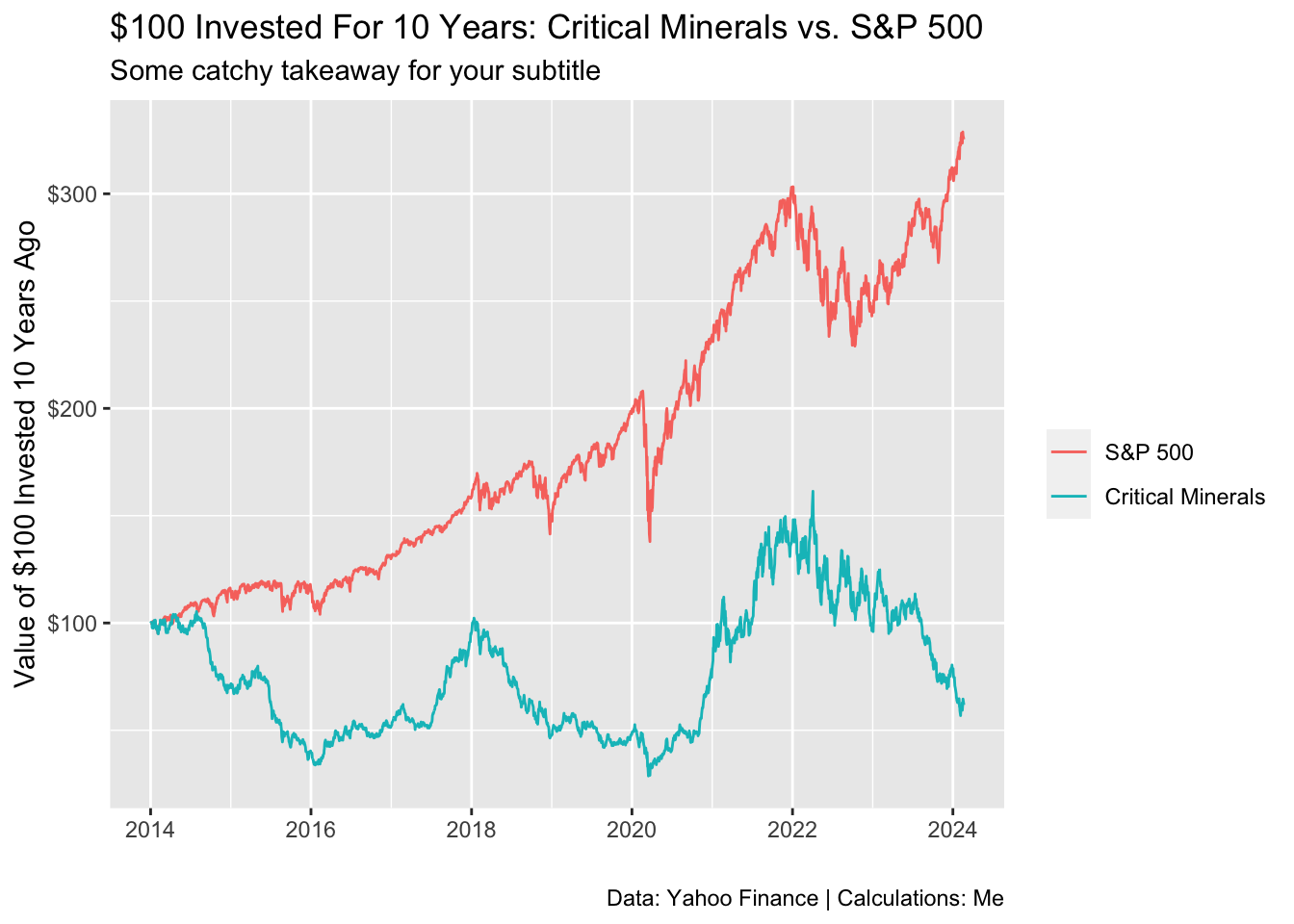
4.5 Practice Problems
4.5.0.1 Homework problem 1:
Your boss knows that they will be asking her about how the implications of the electric vehicle (EV) market and policy choices on the demand for copper and cobalt.
Use the workflow developed in this chapter to import and tidy worksheet
2.3 EVfrom the dataset.Use the tidied dataset to come up with 5 compelling data visualizations that illustrate key actionable insights about how policy scenarios, and technological scenarios will impact demand for copper and cobalt.
Data import is time consuming when you’re first learning, so we’re limiting this to one practice question. Make your insights awesome.
4.6 Resources for Learning More
The Import section of R4DS (2e) has chapters on other data import topics, such as databases, and web scraping.
For sustainable finance related data, Our World in Data is an outstanding resource. They have great open-access datasets on emissions, and on energy that are worth exploring in detail!
The tidyquant package, used above, is a great tool for data import. Check out the documentation here. It automatically tidies the data for you, which is lovely. Here are a few relevant sources it can pull from:
Free financial data from Yahoo Finance. We saw this above. It’s mostly equities data. But hey, it’s free, which is amazing.
Economic and financial data from the Federal Reserve (FRED).
Bloomberg. If, in a professional role, you have access to Bloomberg (very much not free), you can use tidyquant to get a universe of financial data.