library(tidyverse) # because, always
library(janitor) # for clean_names() - makes variable names snake_case3 Data Tidying
3.1 Learning Objectives
You’ll build the foundations of a toolkit for tidying and analyzing sustainable finance data.
Through practical application, you’ll learn to appreciate why data tidying is an important first step that enables you to quickly and seamlessly apply
tidyversetools to make sense of your data and visualize it.You will master
pivot_longer()andpivot_wider()as powerful tools to tidy your data and extract meaningful insights.
3.2 R for Data Science 2e Chapter
Work through the R for Data Science 2e Chapter
The rest of this chapter assumes you’ve read through R for Data Science (2e) Chapter 5 - Data tidying. Run the code as you read. We highly suggest doing the exercises at the end of each section to make sure you understand the concepts. The rest of this chapter in this textbook will assume this knowledge and build upon it to learn about Sustainable Finance applications.
3.3 Resources
3.3.1 Cheatsheet
Print, download, or bookmark the tidyr cheatsheet. Spend a few minutes getting to know it. This cheatsheet will save you a lot of time later.
3.3.2 Package Documentation
The tidyr package website provides extensive documentation of the package’s function and usage.
3.4 Applying Chapter Lessons to Sustainable Finance
3.4.1 Understanding International Issuance of Green Bonds
The green bond market has grown rapidly. With a green bond, the bond’s use of proceeds are tied to a specific environmental expenditure. The IMF’s Climate Change Dashboard has a dataset on green debt that enables us to explore the growth of the green bond market around the world.
We’ll explore three dimensions of the green bond market:
Size: We can understand order of magnitude. Is it a $10 billion market, a $100 billion market, or a $1 trillion market?
Time: The data is presented on a yearly basis, so we can explore growth over time.
Geography: What countries and regions are the largest issuers of green bonds?
3.4.2 Data Tidying Playbook
Before we dive into the data, let’s understand the playbook. This chapter builds on the content in the R4DS chapter to show you how data pivoting is a powerful tool for finding meaning in data. It’s not intuitive, but once you learn it, you’ll never look back.
Tidy untidy data: making our data tidy enables us to quickly and easily transform, model, and visualize our data. The most common form of untidy data we will encounter is time series data where dates (observations) are column headers (variables). Tidying data generally involves using
tidyr::pivot_longer()to take columns that are observations and pivot them into rows (…observations should always be rows).Use
pivot_wider()andpivot_longer()as power tools to find meaning in our dataWe will pivot data wider to use
mutate()to create new useful variables.Then, we will pivot that data longer again and use
group_by()to perform analysis by group usingdplyrtools likemutate(),filter(),slice_*(), andsummarize().Then we’ll
pivot_wider()again and compare groups usingmutate()
This sounds confusing when discussed in the abstract. We’ll dive into examples below that make it real.
Spend Quality Time with the
pivot_*() Documentation
Pivoting is not intuitive.
It takes time and practice. And it’s worth it. Run ?pivot_longer() and ?pivot_wider() and spend time reading the function documentation and running the examples. Both functions have numerous additional arguments you can use beyond the ones necessary to do the basic pivots. No need to memorize these, but it is good to know that they exist, because they will save you time and mental effort later.
3.4.3 Data Set-up
3.4.3.1 Load Packages
As always, we start by loading the packages we’ll be using.
Messages and Warnings
To keep the text clean, this textbook suppresses many of the messages and warnings that pop up when you load packages and data. You will see these messages and warnings. Most warnings are not bad. They are simply trying to give you relevant information. Read them and understand what they are saying. Ask ChatGPT or Google to explain them to you if it’s not readily apparent.
3.4.3.2 Read in Data from IMF Climate Finance Dashboard
Read in the .csv file directly from the internet.
imf_climate_dashboards_green_debt_url <- "https://opendata.arcgis.com/datasets/8e2772e0b65f4e33a80183ce9583d062_0.csv"

green_debt <- imf_climate_dashboards_green_debt_url |>
  read_csv()

green_debt
# A tibble: 355 × 42
ObjectId Country ISO2 ISO3 Indicator Unit Source CTS_Code CTS_Name
<dbl> <chr> <chr> <chr> <chr> <chr> <chr> <chr> <chr>
1 1 Argentina AR ARG Green Bo… Bill… Refin… ECFFI Green B…
2 2 Australia AU AUS Green Bo… Bill… Refin… ECFFI Green B…
3 3 Austria AT AUT Green Bo… Bill… Refin… ECFFI Green B…
4 4 Austria AT AUT Sovereig… Bill… Refin… ECFF Green B…
5 5 Bangladesh BD BGD Green Bo… Bill… Refin… ECFFI Green B…
6 6 Belarus, Rep. … BY BLR Green Bo… Bill… Refin… ECFFI Green B…
7 7 Belarus, Rep. … BY BLR Sovereig… Bill… Refin… ECFF Green B…
8 8 Belgium BE BEL Green Bo… Bill… Refin… ECFFI Green B…
9 9 Belgium BE BEL Sovereig… Bill… Refin… ECFF Green B…
10 10 Bermuda BM BMU Green Bo… Bill… Refin… ECFFI Green B…
# ℹ 345 more rows
# ℹ 33 more variables: CTS_Full_Descriptor <chr>, Type_of_Issuer <chr>,
# Use_of_Proceed <chr>, Principal_Currency <chr>, F1985 <dbl>, F1986 <dbl>,
# F1987 <dbl>, F1990 <dbl>, F1991 <dbl>, F1992 <dbl>, F1993 <dbl>,
# F1994 <dbl>, F1999 <dbl>, F2000 <dbl>, F2002 <dbl>, F2003 <dbl>,
# F2004 <dbl>, F2007 <dbl>, F2008 <dbl>, F2009 <dbl>, F2010 <dbl>,
# F2011 <dbl>, F2012 <dbl>, F2013 <dbl>, F2014 <dbl>, F2015 <dbl>, …This dataset has 42 columns, and 355 rows.
To avoid getting lost in clutter, we’ll create a subset of the data with just the variables we’ll be working with. Here are the steps we’ll take to do that:
filter()for only the indicators we want, using a vectorc()of indicators.janitor::clean_names()converts variable names intosnake_case, which makes them significantly easier to work with in dplyr.select()the variables we want to use. Looking at the data, you’ll notice that the years are represented likeF2008. We’ll use the magic of regular expressions (regex) to select all of those usingmatches("f\d{4}"))
# we want to compare these two indicators
indicators_we_want <- c("Green Bond Issuances by Country", "Sovereign Green Bond Issuances")

green_debt_subset <- green_debt |>
  # from the janitor package -- makes variables snake_case so they are easier to work with
  clean_names() |>
  # filter for the vector of indicators we defined above
  filter(indicator %in% indicators_we_want) |>
  # "f\\d{4}" is a regular expression (regex) that searches for all columns that are f + four digits.
  # Ask ChatGPT to explain this to you.
  select(country, iso3, indicator, matches("f\\d{4}"))

green_debt_subset
# A tibble: 107 × 32
country iso3 indicator f1985 f1986 f1987 f1990 f1991 f1992 f1993 f1994 f1999
<chr> <chr> <chr> <dbl> <dbl> <dbl> <dbl> <dbl> <dbl> <dbl> <dbl> <dbl>
1 Argent… ARG Green Bo… NA NA NA NA NA NA NA NA NA
2 Austra… AUS Green Bo… NA NA NA NA NA NA NA NA NA
3 Austria AUT Green Bo… NA NA NA NA NA NA NA NA NA
4 Austria AUT Sovereig… NA NA NA NA NA NA NA NA NA
5 Bangla… BGD Green Bo… NA NA NA NA NA NA NA NA NA
6 Belaru… BLR Green Bo… NA NA NA NA NA NA NA NA NA
7 Belaru… BLR Sovereig… NA NA NA NA NA NA NA NA NA
8 Belgium BEL Green Bo… NA NA NA NA NA NA NA NA NA
9 Belgium BEL Sovereig… NA NA NA NA NA NA NA NA NA
10 Bermuda BMU Green Bo… NA NA NA NA NA NA NA NA NA
# ℹ 97 more rows
# ℹ 20 more variables: f2000 <dbl>, f2002 <dbl>, f2003 <dbl>, f2004 <dbl>,
# f2007 <dbl>, f2008 <dbl>, f2009 <dbl>, f2010 <dbl>, f2011 <dbl>,
# f2012 <dbl>, f2013 <dbl>, f2014 <dbl>, f2015 <dbl>, f2016 <dbl>,
# f2017 <dbl>, f2018 <dbl>, f2019 <dbl>, f2020 <dbl>, f2021 <dbl>,
# f2022 <dbl>We keep the iso3 country codes because they make it easy to add all sorts of useful information like regions and sub-regions using the countrycode R package.
3.4.4 Step 1: Tidy untidy data
Let’s remember the three rules of tidy data:
There are three interrelated rules that make a dataset tidy:
Each variable is a column; each column is a variable.
Each observation is a row; each row is an observation.
Each value is a cell; each cell is a single value.
Our dataset is presented in wide format. The metadata columns (country, variable type, etc.) are on the left. On the right, each year (an observation) is a column. This wide presentation of time series data is common in economics and finance. It is intuitive for humans to look at. But it is bad for doing data analysis. It violates rule #1 in the list above.
We’ll fix this by using pivot_longer() to take all of the year observations and pivot them into observations (rows) in a column of years.
The only necessary argument is to specify the cols we want to pivot longer. Again, we use the magic of regular expressions to select all columns with an f followed by four digits (e.g. f2015).
green_debt_subset |>
  pivot_longer(
    cols = matches("f\\d{4}")
  )
# A tibble: 3,103 × 5
country iso3 indicator name value
<chr> <chr> <chr> <chr> <dbl>
1 Argentina ARG Green Bond Issuances by Country f1985 NA
2 Argentina ARG Green Bond Issuances by Country f1986 NA
3 Argentina ARG Green Bond Issuances by Country f1987 NA
4 Argentina ARG Green Bond Issuances by Country f1990 NA
5 Argentina ARG Green Bond Issuances by Country f1991 NA
6 Argentina ARG Green Bond Issuances by Country f1992 NA
7 Argentina ARG Green Bond Issuances by Country f1993 NA
8 Argentina ARG Green Bond Issuances by Country f1994 NA
9 Argentina ARG Green Bond Issuances by Country f1999 NA
10 Argentina ARG Green Bond Issuances by Country f2000 NA
# ℹ 3,093 more rowsWe can then use pivot_longer() ’s voluntary arguments to do some useful things:
Give the new columns more descriptive names than the default
nameandvalue.Parse the years using
readr::parse_number(), which turns the string"f2222"into the numeric value2222. Once this column is numeric, we can filter it like a number to select only certain years, and other useful things.We’ll drop
NAvalues, for now. Green bonds are new. Not much use in havingNAvalues from the 1980s.
green_bonds_tidy <- green_debt_subset |>
  pivot_longer(
    # select all coluns with f + 4 numbers
    cols = matches("f\\d{4}"),

    # change from default ("names")
    names_to = "year",
    # same with the values
    values_to = "issuance_bn_usd",

    # readr::parse_number is a handy function that changes the character string
    # "f2222" into the number 2222. Very useful!
    names_transform = readr::parse_number,

    # green bonds are new-ish, we can drop all those NA values in the 80s and 90s for now.
    values_drop_na = TRUE
  )

green_bonds_tidy
# A tibble: 465 × 5
country iso3 indicator year issuance_bn_usd
<chr> <chr> <chr> <dbl> <dbl>
1 Argentina ARG Green Bond Issuances by Country 2017 0.974
2 Argentina ARG Green Bond Issuances by Country 2020 0.0500
3 Argentina ARG Green Bond Issuances by Country 2021 0.916
4 Argentina ARG Green Bond Issuances by Country 2022 0.207
5 Australia AUS Green Bond Issuances by Country 2014 0.526
6 Australia AUS Green Bond Issuances by Country 2015 0.413
7 Australia AUS Green Bond Issuances by Country 2016 0.531
8 Australia AUS Green Bond Issuances by Country 2017 2.53
9 Australia AUS Green Bond Issuances by Country 2018 2.22
10 Australia AUS Green Bond Issuances by Country 2019 1.98
# ℹ 455 more rowsNow we have a tidy dataset! All columns are variables. All rows are observations.
3.4.5 Step 2: Use group_by() Plus dplyr functions to extract meaning
Our two indicators show the issuance of green bonds per country, per year, in billions of USD. We can also calculate the cumulative total of issuance per country in each year.
green_bonds_tidy_cumulative <- green_bonds_tidy |>
  # we don't need that here. get rid of clutter.
  select(-iso3) |>
  # when calculating cumulative totals, make sure the years are in order first
  arrange(country, year) |>
  group_by(country, indicator) |>
  mutate(cumulative_bn_usd = cumsum(issuance_bn_usd)) |>
  # when in doubt, always ungroup after group_by() functions.  Will stop weird behavior.
  ungroup()

green_bonds_tidy_cumulative
# A tibble: 465 × 5
country indicator year issuance_bn_usd cumulative_bn_usd
<chr> <chr> <dbl> <dbl> <dbl>
1 Argentina Green Bond Issuances by Co… 2017 0.974 0.974
2 Argentina Green Bond Issuances by Co… 2020 0.0500 1.02
3 Argentina Green Bond Issuances by Co… 2021 0.916 1.94
4 Argentina Green Bond Issuances by Co… 2022 0.207 2.15
5 Australia Green Bond Issuances by Co… 2014 0.526 0.526
6 Australia Green Bond Issuances by Co… 2015 0.413 0.938
7 Australia Green Bond Issuances by Co… 2016 0.531 1.47
8 Australia Green Bond Issuances by Co… 2017 2.53 4.00
9 Australia Green Bond Issuances by Co… 2018 2.22 6.22
10 Australia Green Bond Issuances by Co… 2019 1.98 8.21
# ℹ 455 more rowsWhen analyzing new data, start by answering basic questions first.
With the cumulative totals we’ve calculated, we can now answer the basic question: what countries are the biggest cumulative issuers of green bonds?
biggest_green_bond_issuers <- green_bonds_tidy_cumulative |>
  filter(indicator == "Green Bond Issuances by Country") |>
  group_by(country) |>
  slice_max(order_by = year) |>
  arrange(cumulative_bn_usd|> desc()) |>
  select(country, cumulative_bn_usd) |>
  ungroup()

biggest_green_bond_issuers
# A tibble: 79 × 2
country cumulative_bn_usd
<chr> <dbl>
1 China, P.R.: Mainland 325.
2 Germany 253.
3 France 213.
4 United States 172.
5 Netherlands, The 155.
6 United Kingdom 84.0
7 Sweden 76.6
8 Spain 65.7
9 Japan 61.8
10 Italy 59.9
# ℹ 69 more rowsEverybody loves a ranked list. And now we have one.
It is not difficult to imagine the work situations in which your future boss, the Finance Minister considering issuing a soveriegn green bond, or the senior banker considering global green bond underwriting opportunities, might want to know this information.
We seek repeatable factoids and insightful data visualizations. What’s better than a ranked list? A top 10 list. What’s better than a top 10 list? A top 10 sorted bar chart.
top_10_chart <- biggest_green_bond_issuers |>

  # take the top 10, ordered by cumulative issuance
  slice_max(order_by = cumulative_bn_usd, n = 10) |>

  ggplot(aes(x = cumulative_bn_usd,
             # order countries by cumulative issuance
             y = fct_reorder(.f = country, .x = cumulative_bn_usd)
             )) +
  geom_col(fill = "forestgreen")

top_10_chart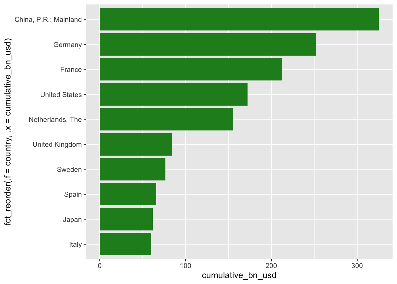
This is a great start for our own consumption. Let’s pretty this up to show our boss.
top_10_chart +
  theme_minimal() +
  scale_x_continuous(labels = scales::label_dollar(suffix = " bn"),
                     expand = c(0,0)) +
  labs(title = "Top 10 Green Bond Issuers",
       subtitle = "The Dutch sure do issue a whole lot of green bonds per capita",
       x = "Cumulative Issuance (USD)",
       y = "",
       caption = "Data: IMF Climate Change Dashboard | Insight: Me!")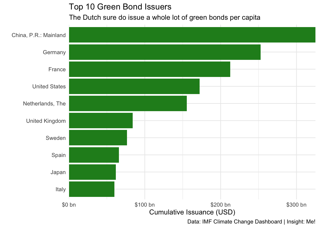
Sorted bar charts provide the viewer clear insight into both ranking and magnitude.
3.4.6 Step 3: pivot_wider() to Create New Variables
Our dataset provides information about sovereign green bond issuances, and about total green bond issuances. Sovereign green bonds are newer. In 2020-2021, your professor co-authored a World Bank paper with a former Chilean Finance Minister who had spearheaded Chile’s sovereign green bond program. How big is the sovereign green bond market now compared to the more established corporate green bond market?
We can estimate corporate green bond issuance by subtracting sovereign green bond issuance from total green bond issuance.1
To do this, we’ll want to pivot_wider() to make the the values in the indicator column into column headers, with the values from the issuance_bn_usd column filled in underneath.
green_bonds_tidy |>
  pivot_wider(names_from = indicator,
              values_from = issuance_bn_usd)
# A tibble: 420 × 5
country iso3 year Green Bond Issuances by Countr…¹ Sovereign Green Bond…²
<chr> <chr> <dbl> <dbl> <dbl>
1 Argentina ARG 2017 0.974 NA
2 Argentina ARG 2020 0.0500 NA
3 Argentina ARG 2021 0.916 NA
4 Argentina ARG 2022 0.207 NA
5 Australia AUS 2014 0.526 NA
6 Australia AUS 2015 0.413 NA
7 Australia AUS 2016 0.531 NA
8 Australia AUS 2017 2.53 NA
9 Australia AUS 2018 2.22 NA
10 Australia AUS 2019 1.98 NA
# ℹ 410 more rows
# ℹ abbreviated names: ¹`Green Bond Issuances by Country`,
# ²`Sovereign Green Bond Issuances`Let’s improve the code:
It’s a pain to work with multi word variable names because you have to remember to surround them by single quotation marks. So we we will make them
snake_caseusingjanitor::clean_names().Second, the values that show up as
NAhere aren’t really missing values in our context — they are years when there has been zero dollars of green bond issuance, so we’ll use thevalues_fillargument to fill in0instead ofNA.Finally, we can calculate our new corporate green bond issuance variable. If you want to sound sophisticated, you can call this step feature engineering.
corporate_vs_sovereign_green_bonds <- green_bonds_tidy |>
  select(-iso3) |>
  pivot_wider(names_from = indicator,
              values_from = issuance_bn_usd,

              values_fill = 0) |>
  clean_names() |>
  mutate(corporate_green_bond_issuances = green_bond_issuances_by_country - sovereign_green_bond_issuances)

corporate_vs_sovereign_green_bonds
# A tibble: 420 × 5
country year green_bond_issuances_by_country sovereign_green_bond_issuan…¹
<chr> <dbl> <dbl> <dbl>
1 Argentina 2017 0.974 0
2 Argentina 2020 0.0500 0
3 Argentina 2021 0.916 0
4 Argentina 2022 0.207 0
5 Australia 2014 0.526 0
6 Australia 2015 0.413 0
7 Australia 2016 0.531 0
8 Australia 2017 2.53 0
9 Australia 2018 2.22 0
10 Australia 2019 1.98 0
# ℹ 410 more rows
# ℹ abbreviated name: ¹sovereign_green_bond_issuances
# ℹ 1 more variable: corporate_green_bond_issuances <dbl>3.4.7 Step 4: Manufacturing Repeatable Factoids Through Pivots
Now that we’ve created the new variable, we’ll
pivot it back into an
indicatorrow usingpivot_longer().Then, we’ll compare two countries by filtering
countryfor those two countries, pivoting them wider.Finally we’ll using
mutate()to calculate comparisons and findrepeatable factoids.
The logic of this step is tricky at first, but once you understand it, you’ll find yourself using it all the time.
3.4.7.1 Step 4.1: Pivot New Variables Longer
First, we want our green bond issuance variables in long form so that we can do grouped analysis.
corporate_vs_sovereign_green_bonds |>
  pivot_longer(cols = contains("green_bond"))
# A tibble: 1,260 × 4
country year name value
<chr> <dbl> <chr> <dbl>
1 Argentina 2017 green_bond_issuances_by_country 0.974
2 Argentina 2017 sovereign_green_bond_issuances 0
3 Argentina 2017 corporate_green_bond_issuances 0.974
4 Argentina 2020 green_bond_issuances_by_country 0.0500
5 Argentina 2020 sovereign_green_bond_issuances 0
6 Argentina 2020 corporate_green_bond_issuances 0.0500
7 Argentina 2021 green_bond_issuances_by_country 0.916
8 Argentina 2021 sovereign_green_bond_issuances 0
9 Argentina 2021 corporate_green_bond_issuances 0.916
10 Argentina 2022 green_bond_issuances_by_country 0.207
# ℹ 1,250 more rowsOur indicator names are still in snake_case, which is ugly if we want to use them in a chart. We’ll use a simple custom function with the names_transform argument of pivot_longer() to transform them back into Title Case (all first letters of words capitalized).
snake_case_to_title_case <- function(input_string) {

  input_string |>
    # Replace underscores with spaces
    str_replace_all(pattern = "_", replacement = " ") |>
    # change capitalization to Title Case
    str_to_title()
}

corporate_vs_sovereign_green_bonds_long <- corporate_vs_sovereign_green_bonds |>
  pivot_longer(cols = contains("green_bond"),
               names_to = "indicator",
               values_to = "issuance_bn_usd",
               names_transform = snake_case_to_title_case)

corporate_vs_sovereign_green_bonds_long
# A tibble: 1,260 × 4
country year indicator issuance_bn_usd
<chr> <dbl> <chr> <dbl>
1 Argentina 2017 Green Bond Issuances By Country 0.974
2 Argentina 2017 Sovereign Green Bond Issuances 0
3 Argentina 2017 Corporate Green Bond Issuances 0.974
4 Argentina 2020 Green Bond Issuances By Country 0.0500
5 Argentina 2020 Sovereign Green Bond Issuances 0
6 Argentina 2020 Corporate Green Bond Issuances 0.0500
7 Argentina 2021 Green Bond Issuances By Country 0.916
8 Argentina 2021 Sovereign Green Bond Issuances 0
9 Argentina 2021 Corporate Green Bond Issuances 0.916
10 Argentina 2022 Green Bond Issuances By Country 0.207
# ℹ 1,250 more rows3.4.7.2 Step 4.2: Select Groups to Compare and Pivot Them Wider
Based upon the data visualization we made above, it looks interesting to compare green bond issuance in China2 and Germany. We can do this by filtering for these two countries, and comparing them over time.
The first step is to pivot the two countries wider into columns.
china_vs_germany_green_bonds <- corporate_vs_sovereign_green_bonds_long |>
  filter(country %in% c("China, P.R.: Mainland", "Germany")) |>
  arrange(year) |>
  pivot_wider(names_from = country,
              values_from = issuance_bn_usd,
              values_fill = 0) |>
  clean_names()

china_vs_germany_green_bonds
# A tibble: 48 × 4
year indicator germany china_p_r_mainland
<dbl> <chr> <dbl> <dbl>
1 1991 Green Bond Issuances By Country 0.0292 0
2 1991 Sovereign Green Bond Issuances 0 0
3 1991 Corporate Green Bond Issuances 0.0292 0
4 1992 Green Bond Issuances By Country 0.0350 0
5 1992 Sovereign Green Bond Issuances 0 0
6 1992 Corporate Green Bond Issuances 0.0350 0
7 1993 Green Bond Issuances By Country 0.0175 0
8 1993 Sovereign Green Bond Issuances 0 0
9 1993 Corporate Green Bond Issuances 0.0175 0
10 2000 Green Bond Issuances By Country 0.0272 0
# ℹ 38 more rows3.4.7.3 Step 4.3: Manufacture Repeatable Factoids Using mutate()
In written and verbal communication, three forms of quantitative comparison will serve you well, depending on the context and magnitude of differences.
Multiples: when the order of magnitude of difference is large, using multiples works best. “X is 40 times bigger than Y”
Percentages: when one group is less than 1x larger than the other, percentage differences are commonly the best form of comparison. “X is 40% smaller than Y”
Absolute Differences: This works well when the audience has an intuitive sense of the sizes discussed. For example, people have an intuitive sense of human heights, so it is meaningful to say that one person is 7 inches (or cm) taller than another. But in our circumstance, there is no reason to think that our audience has an intuitive sense of whether $2 billion of green bond issuance between two countries is large or small. “X is $2 million more than Y”
Let’s set ourselves up for success by calculating comparisons in both directions. Make the variable names descriptive so that you know what you’re looking at later. Don’t worry about variable names being long.
china_vs_germany_green_bonds_repeatable_factoids <- china_vs_germany_green_bonds |>
  mutate(

    # multiples:
    # "Germany issued x times more than China"
    germany_x_than_china = germany/china_p_r_mainland,
    # "China issued x times more than Germany"
    china_x_than_germany = china_p_r_mainland/germany,

    # percent more:
    # "Germany issued x% more than China"
    germany_pct_more_than_china = (germany/china_p_r_mainland-1) * 100,
    # "China issued x% more than Germany"
    china_pct_more_than_germany = (china_p_r_mainland/germany-1) * 100

    # could do absolute difference, etc.... anything that makes intuitive sense.

         )

china_vs_germany_green_bonds_repeatable_factoids
# A tibble: 48 × 8
year indicator germany china_p_r_mainland germany_x_than_china
<dbl> <chr> <dbl> <dbl> <dbl>
1 1991 Green Bond Issuances B… 0.0292 0 Inf
2 1991 Sovereign Green Bond I… 0 0 NaN
3 1991 Corporate Green Bond I… 0.0292 0 Inf
4 1992 Green Bond Issuances B… 0.0350 0 Inf
5 1992 Sovereign Green Bond I… 0 0 NaN
6 1992 Corporate Green Bond I… 0.0350 0 Inf
7 1993 Green Bond Issuances B… 0.0175 0 Inf
8 1993 Sovereign Green Bond I… 0 0 NaN
9 1993 Corporate Green Bond I… 0.0175 0 Inf
10 2000 Green Bond Issuances B… 0.0272 0 Inf
# ℹ 38 more rows
# ℹ 3 more variables: china_x_than_germany <dbl>,
# germany_pct_more_than_china <dbl>, china_pct_more_than_germany <dbl>Use your growing domain expertise and curiousity to look for patterns that stand out to you. Here are two points of comparison that stand out to me when I look through the data.
factoid_2014 <- china_vs_germany_green_bonds_repeatable_factoids |>
  filter(year == 2014) |>
  filter(indicator == "Green Bond Issuances By Country") |>
  pull(germany_x_than_china) |>
  round()

factoid_2014
[1] 25factoid_2022 <- china_vs_germany_green_bonds_repeatable_factoids |>
filter(year == 2022) |>
filter(indicator == "Green Bond Issuances By Country") |>
pull(china_pct_more_than_germany) |>
round()
factoid_2022[1] 19Here’s our repeatable factoid:
“In 2014, Germany issued 25 times more green bonds than China. By 2022, China issued 19% more green bonds than Germany.”
In the quote above, the numbers are not hard coded, they are inserted from the variables above using inline code in Quarto. That means if the numbers were updated in the data, they would automatically update in the text.

Imagine how much easier this functionality could make the presentation you have to update every week?
3.5 Practice Problems
3.5.0.1 Homework problem 1:
Use the
countrycodepackage to add the region as a variable togreen_debt_subset.Calculate the cumulative issuance of green bonds by region.
Use
ggplot2to make a data visualization comparing regional cumulative issuance.Make your plot look professionally presentable, as we did above.
3.5.0.2 Homework problem 2:
Use the full
green_debt datasetUse
clean_names()to make the variable names snake_caseFilter out observations where
type_of_issueris “Not Applicable”Use the tools taught in this chapter to provide a compelling data visualization and some repeatable factoids that provide actionable insights about green bond issuers.
3.5.0.3 Homework problem 3:
Repeat the process from problem 2 for
use_of_proceedand forprincipal_currencyWhat are green bond proceeds used for?
What do we know about the currency of issuance? Is that changing over time?
green_debt |>
  clean_names() |>
  filter(type_of_issuer != "Not Applicable")
# A tibble: 7 × 42
object_id country iso2 iso3 indicator unit source cts_code cts_name
<dbl> <chr> <chr> <chr> <chr> <chr> <chr> <chr> <chr>
1 347 World <NA> WLD Green Bond Issua… Bill… Refin… ECFFI Green B…
2 348 World <NA> WLD Green Bond Issua… Bill… Refin… ECFFI Green B…
3 349 World <NA> WLD Green Bond Issua… Bill… Refin… ECFFI Green B…
4 350 World <NA> WLD Green Bond Issua… Bill… Refin… ECFFI Green B…
5 351 World <NA> WLD Green Bond Issua… Bill… Refin… ECFFI Green B…
6 352 World <NA> WLD Green Bond Issua… Bill… Refin… ECFFI Green B…
7 353 World <NA> WLD Green Bond Issua… Bill… Refin… ECFFI Green B…
# ℹ 33 more variables: cts_full_descriptor <chr>, type_of_issuer <chr>,
# use_of_proceed <chr>, principal_currency <chr>, f1985 <dbl>, f1986 <dbl>,
# f1987 <dbl>, f1990 <dbl>, f1991 <dbl>, f1992 <dbl>, f1993 <dbl>,
# f1994 <dbl>, f1999 <dbl>, f2000 <dbl>, f2002 <dbl>, f2003 <dbl>,
# f2004 <dbl>, f2007 <dbl>, f2008 <dbl>, f2009 <dbl>, f2010 <dbl>,
# f2011 <dbl>, f2012 <dbl>, f2013 <dbl>, f2014 <dbl>, f2015 <dbl>,
# f2016 <dbl>, f2017 <dbl>, f2018 <dbl>, f2019 <dbl>, f2020 <dbl>, …3.6 Resources for Learning More
This chapter has focused on the pivot_*() functions, which are only one set of tools from tidyr. Learning the full tidyr toolkit will enable you to clean your data painlessly and get to the fun stuff quicker.
Beyond the resources listed at the top of the chapter, here are a few resources to learn more:
This estimate will not be exact. There are green municipal and sub-national bonds that are neither sovereign or corporate. But it should be a pretty good estimate, as corporate issuance is likely orders of magnitude larger than these other non-sovereign issuance. In a more in-depth analysis, you would want to investigate this.↩︎
The dataset has separate entries for Hong Kong and Macao. Depending on the context of the analysis, one could lump those together to get a more complete picture of Chinese green bond issuance. Here, we keep it simple.↩︎