2 Data Transformation

2.1 Learning Objectives

In this chapter, you will:

Enhance your knowledge of dplyr’s grammar by using its verbs (filter, mutate , select , summarize , group_by, and the minor verbs) to analyze sustainable finance data.
Learn and practice strategies for uncovering meaningful insights from sustainable finance data using data transformation.
You will practice communicating your findings to others using data visualizations and repeatable factoids.

2.2 R for Data Science 2e Chapter

Work through the R for Data Science 2e Chapter

The rest of this chapter assumes you’ve read through R for Data Science Chapter (2e) 3 - Data transformation. Run the code as you read. We highly suggest doing the exercises at the end of each section to make sure you understand the concepts. The rest of this chapter in this textbook will assume this knowledge and build upon it to learn about Sustainable Finance applications.

R for Data Science Chapter (2e) 3 - Data transformation:

2.3 Resources

2.3.1 Cheatsheet

Print, download, or bookmark the dplyr cheatsheet. Spend a few minutes getting to know it. This cheatsheet will save you a lot of time later.

dplyr cheatsheet:

2.3.2 Package Documentation

The dplyr package website provides extensive documentation of the package’s function and usage.

dplyr package website:

2.3.3 Mind Map

This mind map visualizes the menu of dplyr’s key functionality for transforming your data.

2.4 Applying Chapter Lessons to Sustainable Finance

BlackRock has trillions of dollars in assets under management in its ETF business. How much of this is in ESG products?

For all the focus on advanced statistics and econometrics in graduate programs, a surprisingly large amount of your time as a professional will be spent using simple tools to extract meaningful insights from big, boring spreadsheets.

The iShares website provides an option to download a spreadsheet, updated regularly, with information about all of their ETF offerings. Let’s use our new data transformation skills to explore BlackRock’s ETF business from another perspective.

2.4.1 Getting started

We always start by loading the necessary packages that we’ll be using. Here we’ve also set the options() for our R session so that it doesn’t return scientific notation (e.g 2.55e12), which can be annoying in our context.

#load the tidyverse 
library(tidyverse)

Warning: package 'ggplot2' was built under R version 4.3.1

── Attaching core tidyverse packages ──────────────────────── tidyverse 2.0.0 ──
✔ dplyr     1.1.4     ✔ readr     2.1.4
✔ forcats   1.0.0     ✔ stringr   1.5.0
✔ ggplot2   3.4.4     ✔ tibble    3.2.1
✔ lubridate 1.9.3     ✔ tidyr     1.3.0
✔ purrr     1.0.2     
── Conflicts ────────────────────────────────────────── tidyverse_conflicts() ──
✖ dplyr::filter() masks stats::filter()
✖ dplyr::lag()    masks stats::lag()
ℹ Use the conflicted package (<http://conflicted.r-lib.org/>) to force all conflicts to become errors

# this will stop R from presenting data in scientific notation, which can be annoying. 
options(scipen = 999)

Read the cleaned data from our class GitHub data repo.

blackrock_etf_screener <- read_csv("https://raw.githubusercontent.com/t-emery/sais-susfin_data/main/datasets/ishares_etf_screener_as_of_2023-12-27.csv") 

blackrock_etf_screener

# A tibble: 424 × 18
   ticker name                        incept_date         gross_expense_ratio_…¹
   <chr>  <chr>                       <dttm>                               <dbl>
 1 IVV    iShares Core S&P 500 ETF    2000-05-15 00:00:00                   0.03
 2 IEFA   iShares Core MSCI EAFE ETF  2012-10-18 00:00:00                   0.07
 3 AGG    iShares Core U.S. Aggregat… 2003-09-22 00:00:00                   0.03
 4 IWF    iShares Russell 1000 Growt… 2000-05-22 00:00:00                   0.19
 5 IJR    iShares Core S&P Small-Cap… 2000-05-22 00:00:00                   0.06
 6 IJH    iShares Core S&P Mid-Cap E… 2000-05-22 00:00:00                   0.05
 7 IEMG   iShares Core MSCI Emerging… 2012-10-18 00:00:00                   0.09
 8 IWM    iShares Russell 2000 ETF    2000-05-22 00:00:00                   0.19
 9 IWD    iShares Russell 1000 Value… 2000-05-22 00:00:00                   0.19
10 TLT    iShares 20+ Year Treasury … 2002-07-22 00:00:00                   0.15
# ℹ 414 more rows
# ℹ abbreviated name: ¹gross_expense_ratio_percent
# ℹ 14 more variables: net_expense_ratio_percent <dbl>, net_assets_usd <dbl>,
#   net_assets_as_of <dttm>, asset_class <chr>, sub_asset_class <chr>,
#   region <chr>, market <chr>, location <chr>, investment_style <chr>,
#   msci_esg_fund_rating_aaa_ccc <chr>, msci_esg_quality_score_0_10 <dbl>,
#   msci_weighted_average_carbon_intensity_tons_co2e_m_sales <dbl>, …

2.4.2 Exploring our Dataset

2.4.2.1 `glimpse()` your dataset

dplyr::glimpse() is a great way to take a first look at your data once you’ve imported it. It shows the column names, column types , and a preview of the first observations of your data.

blackrock_etf_screener |> 
  glimpse()

Rows: 424
Columns: 18
$ ticker                                                   <chr> "IVV", "IEFA"…
$ name                                                     <chr> "iShares Core…
$ incept_date                                              <dttm> 2000-05-15, …
$ gross_expense_ratio_percent                              <dbl> 0.03, 0.07, 0…
$ net_expense_ratio_percent                                <dbl> 0.03, 0.07, 0…
$ net_assets_usd                                           <dbl> 399312542067,…
$ net_assets_as_of                                         <dttm> 2023-12-27, …
$ asset_class                                              <chr> "Equity", "Eq…
$ sub_asset_class                                          <chr> "Large Cap", …
$ region                                                   <chr> "North Americ…
$ market                                                   <chr> "Developed", …
$ location                                                 <chr> "United State…
$ investment_style                                         <chr> "Index", "Ind…
$ msci_esg_fund_rating_aaa_ccc                             <chr> "A", "AA", "A…
$ msci_esg_quality_score_0_10                              <dbl> 6.6845, 7.519…
$ msci_weighted_average_carbon_intensity_tons_co2e_m_sales <dbl> 106.80, 102.8…
$ msci_esg_percent_coverage                                <dbl> 99.05, 99.80,…
$ sustainable_classification                               <chr> NA, NA, NA, N…

2.4.2.2 Exploring categorical variables, 3 ways using `dplyr`

Given that we’re trying to uncover meaningful insights related to sustainable finance, sustainable_classification is a natureal starting point. Let’s find its distinct levels using distinct().

blackrock_etf_screener |> 
  distinct(sustainable_classification)

# A tibble: 5 × 1
  sustainable_classification
  <chr>                     
1 <NA>                      
2 Uplift                    
3 Thematic                  
4 Impact                    
5 Screened

We see that there are 4 types of fund classifications, and NA values.

How many NA values are there? And how many Impact funds? We can use count() to find this out.

blackrock_etf_screener |> 
  group_by(sustainable_classification) |> 
  count(sort = TRUE)

# A tibble: 5 × 2
# Groups:   sustainable_classification [5]
  sustainable_classification     n
  <chr>                      <int>
1 <NA>                         384
2 Uplift                        30
3 Thematic                       6
4 Screened                       3
5 Impact                         1

That gives us a lot more context. There are a lot of NA values. Given the context of the dataset, we can assume that NA values are funds that are “Standard” (non ESG) funds that don’t have sustainable classifications.

We follow the money, so knowing the number of funds is only partially satisfying. What are the total assets in each grouping?

We can use summarize() to find out.

blackrock_etf_screener |> 
  group_by(sustainable_classification) |> 
  summarize(
    # how many funds?
    n_funds = n(),
    # how much money?
    assets_usd = sum(net_assets_usd, na.rm = TRUE)
    ) |> 
  # arrange in descending order
  arrange(assets_usd |> desc())

# A tibble: 5 × 3
  sustainable_classification n_funds assets_usd
  <chr>                        <int>      <dbl>
1 <NA>                           384    2.55e12
2 Uplift                          30    5.14e10
3 Thematic                         6    3.43e 9
4 Screened                         3    3.83e 8
5 Impact                           1    3.35e 8

We’ve already learned a lot from a few simple data transformations. There’s only 1 Impact fund. It doesn’t have a lot of assets. The large bulk of ESG assets are in Uplift funds. What are Uplift funds? We can explore the website to read about what exactly that means and how it differs from Thematic, Screened, and Impact funds.

Three points arise from this initial analysis that we can pursue:

Standard vs. ESG: It’s best to start analysis broad and go progressively deeper. Looking at ESG funds as a whole is more meaningful initially than looking at Uplift, Thematic, or any detailed breakdown.
Time: ESG is relatively new. How has this changed over time?
Money magnitude: $2,547,421,888,526 sure seems like a lot of money. But without literally counting the commas, can you tell whether it is millions, billions, or trillions?

Let’s work on these using mutate()

2.4.3 Feature Engineering with `mutate()`

Feature engineering is the process of creating new variables from our raw data that will be useful in analysis or modeling. The term is commonly used in the context of machine learning, but it is equally relevant to exploratory analysis we’re doing here.

We’re going to address the issues discussed above by creating three new variables:

standard_or_esg that will label a fund as Standard if there is an NA in the sustainable_classification column, and ESG if not.
inception_year that extracts the year from incept_date.
net_assets_bn_usd that transforms net_assets_usd into a magnitude meaningful for our analysis by dividing by $10^9$ (1 billion).

blackrock_etf_screener_w_new_features <- blackrock_etf_screener |> 
  mutate(
    # if the sustainable_classification column is NA, then the fund is not an ESG fund.
    standard_or_esg = if_else(
      condition = is.na(sustainable_classification),
      true = "Standard",
      false = "ESG"
    ),
    # lubridate::year() extracts the year from a date
    inception_year = lubridate::year(incept_date),
    
    # Change to a meaningful magnitude for the data. In asset management, billions is a good default. 
    net_assets_bn_usd = net_assets_usd/10^9,
    
    # let's put our new variables at the front so we can see them easily.
    .before = everything()
  )

blackrock_etf_screener_w_new_features

# A tibble: 424 × 21
   standard_or_esg inception_year net_assets_bn_usd ticker name                 
   <chr>                    <dbl>             <dbl> <chr>  <chr>                
 1 Standard                  2000             399.  IVV    iShares Core S&P 500…
 2 Standard                  2012             107.  IEFA   iShares Core MSCI EA…
 3 Standard                  2003             101.  AGG    iShares Core U.S. Ag…
 4 Standard                  2000              82.1 IWF    iShares Russell 1000…
 5 Standard                  2000              78.2 IJR    iShares Core S&P Sma…
 6 Standard                  2000              77.1 IJH    iShares Core S&P Mid…
 7 Standard                  2012              73.9 IEMG   iShares Core MSCI Em…
 8 Standard                  2000              67.7 IWM    iShares Russell 2000…
 9 Standard                  2000              55.4 IWD    iShares Russell 1000…
10 Standard                  2002              52.2 TLT    iShares 20+ Year Tre…
# ℹ 414 more rows
# ℹ 16 more variables: incept_date <dttm>, gross_expense_ratio_percent <dbl>,
#   net_expense_ratio_percent <dbl>, net_assets_usd <dbl>,
#   net_assets_as_of <dttm>, asset_class <chr>, sub_asset_class <chr>,
#   region <chr>, market <chr>, location <chr>, investment_style <chr>,
#   msci_esg_fund_rating_aaa_ccc <chr>, msci_esg_quality_score_0_10 <dbl>,
#   msci_weighted_average_carbon_intensity_tons_co2e_m_sales <dbl>, …

2.4.4 Analyzing ESG vs. Standard Funds

Two helpful rules of thumb:

In exploratory analysis, start broad. Then get specific.
In finance, it’s always clear where to look first. Follow the money.

Following this guidance, let’s start by calculating the total net assets of all iShares funds.

blackrock_etf_screener_w_new_features |> 
  summarize(total_assets_bn = sum(net_assets_bn_usd, na.rm = TRUE))

# A tibble: 1 × 1
  total_assets_bn
            <dbl>
1           2603.

BlackRock iShares funds have total assets of $2603 billion. Any time you go into four digits, it’s best to resize the number to the next magnitude by dividing by $10^3$. It sounds a lot smoother to say that $2.6 trillion.

Magnitude Switching $$$

Always present your dollar figures in a magnitude that will be intuitive for your audience. During analysis you’ll be aggregating and disaggregating numbers frequently. Here’s a simple tip for changing magnitudes.

$10^0$ = 1 = one

$10^3$ = 1,000 = one thousand

$10^6$ = 1,000,000 = one million

$10^9$ = 1,000,000,000 = one billion

$10^{12}$ = 1,000,000,000,000 = one trillion

Larger magnitude to smaller magnitude: If you are going from a number in trillions ($10^{12}$ ), such as a large country’s GDP, to a number in the thousands ($10^3$ ), such as that country’s per capita GDP, take the following steps:

subtract the exponents: 12 - 3 = 9. Then multiply by 10 to that exponent (9).

$0.000000027 trillion * $10^9$ = $27 thousand

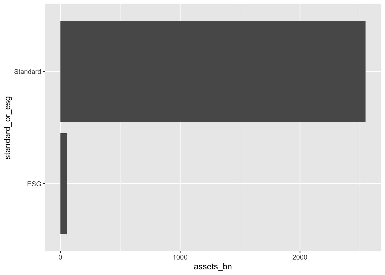
Smaller magnitude to larger magnitude: We saw this above. Assets in standard ETFs were $2,547,421,888,526 . This is expressed in units of 1 ($10^0$), when it really makes sense to express it in trillions ($10^{12}$).

subtract the expontents: 0-12 = -12. Then multpily by 10 to that exponent (-12). Multiplying by a negative exponent is the same as dividing, so do it whichever way you prefer.

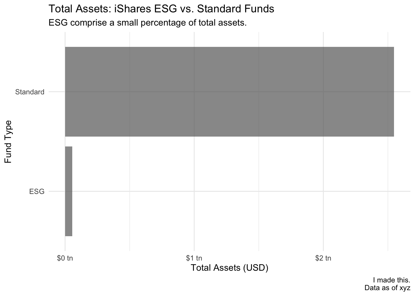
$2,547,421,888,526 * $10^{-12}$ = $2.5 trillion

2.4.4.1 Static Analysis: How big a share is the ESG business?

Analyzing relative size is a central theme of exploratory analysis. There are two related questions.

Static: What is the size right now?
Dynamic: Is it growing or shrinking over time?

We’ll start with a static analysis of the relative size of ESG and Standard funds.

assets_esg_vs_standard <- blackrock_etf_screener_w_new_features |> 
  group_by(standard_or_esg) |> 
  summarize(
    assets_bn = sum(net_assets_bn_usd, na.rm = TRUE),
    n_funds = n()
    )

assets_esg_vs_standard

# A tibble: 2 × 3
  standard_or_esg assets_bn n_funds
  <chr>               <dbl>   <int>
1 ESG                  55.6      40
2 Standard           2547.      384

Our brains understand pictures more intuitively than numbers. Let’s make a quick exploratory chart.

assets_esg_vs_standard |> 
  ggplot(aes(x = assets_bn, y = standard_or_esg)) +
  geom_bar(stat = "identity")

Oh my. That’s notable. We might want to show this to our colleagues or our boss.

We look for two types of outputs to share with others:

Repeatable factoids: Our job is to cut through the noise and present people with a few facts about our data that will resonate and are likely to to be repeated if they were to explain what you told them to others.
Well-formatted data visualizations: The chart above is perfectly fine for your own viewing. But if you’re going to share it with anyone else, at a minimum 1) make the axis units clear, 2) give informative titles and labels so your viewers know what they are looking at.

Above, we see that ESG ETFs make up a small proportion of total assets. But what is the exact percentage? We can find this out using mutate().

assets_esg_vs_standard |> 
  mutate(assets_pct = assets_bn/sum(assets_bn) * 100,
         .after = standard_or_esg)

# A tibble: 2 × 4
  standard_or_esg assets_pct assets_bn n_funds
  <chr>                <dbl>     <dbl>   <int>
1 ESG                   2.14      55.6      40
2 Standard             97.9     2547.      384

Here’s a repeatable factoid:

“ESG assets account for 2.14 % of iShares net assets.”

Now lets make a chart that we can share with our colleagues.

assets_esg_vs_standard |> 
  ggplot(aes(x = assets_bn, y = standard_or_esg)) +
  geom_bar(stat = "identity", fill = "grey40", alpha = .7) +
  
  # make it prettier
  # scales::label_* funcitons provide useful options. Check them out!
  scale_x_continuous(labels = scales::label_dollar(scale = 1/10^3, suffix = " tn")) +
  labs(title = "Total Assets: iShares ESG vs. Standard Funds",
       subtitle = "ESG comprise a small percentage of total assets.",
       x = "Total Assets (USD)",
       y = "Fund Type",
       # you can use \n to create a line break
       caption = "I made this.\nData as of xyz") +
  theme_minimal()

2.4.4.2 Dynamic Analysis: is ESG growing or shrinking over time?

In an ideal world, we’d have a well-formatted time series with assets over time. But this is not an ideal world. We work with the data that is available.

The iShares excel workbook has the start date for each fund (incept_date). We’ve extracted the year in our column inception_year). This provides insights into fund launches. We know from our static analysis that ESG funds are (so far) a small proportion of overall fund assets. What is the pace of ESG fund launches? How does that compare to Standard funds?

etf_formation_esg_vs_standard <- blackrock_etf_screener_w_new_features |> 
  group_by(standard_or_esg, inception_year) |> 
  count() |> 
  ungroup()

etf_formation_esg_vs_standard

# A tibble: 37 × 3
   standard_or_esg inception_year     n
   <chr>                    <dbl> <int>
 1 ESG                       2005     1
 2 ESG                       2006     1
 3 ESG                       2008     1
 4 ESG                       2014     1
 5 ESG                       2016     5
 6 ESG                       2017     2
 7 ESG                       2018     3
 8 ESG                       2019     1
 9 ESG                       2020    12
10 ESG                       2021     5
# ℹ 27 more rows

It’s useful to look at this data using multiple data visualizations, because they will each highlight something slightly different.

A stacked bar chart is useful because it shows you both the overall trend (all fund launches), as well as providing a visual breakdown by fund type.

etf_formation_esg_vs_standard |> 
  ggplot(aes(x = inception_year, y = n, fill = standard_or_esg)) +
  geom_bar(stat = "identity", position = "stack")

We see that ESG funds first show up in 2005. We see a very small number until 2016, when there is a significant uptick in ESG fund launches. In 2023 there was a large number of fund launches, but only a few were ESG funds.

Here’s another way to display the data that is better for comparing a category against itself, and against other categories (at the expense of not showing the aggregate well).

etf_formation_esg_vs_standard |> 
  ggplot(aes(x = inception_year, y = n, color = standard_or_esg)) +
  geom_line()

Cumulative aggregates, using cumsum() can also uncover interesting trends. You want to make sure your data are in the order you’d like them to be. In our case that means we want to arrange() the years in ascending order.

etf_formation_esg_vs_standard_cumulative <- etf_formation_esg_vs_standard |> 
  arrange(standard_or_esg, inception_year) |> 
  group_by(standard_or_esg) |> 
  mutate(cumulative_n = cumsum(n)) |> 
  ungroup()

etf_formation_esg_vs_standard_cumulative

# A tibble: 37 × 4
   standard_or_esg inception_year     n cumulative_n
   <chr>                    <dbl> <int>        <int>
 1 ESG                       2005     1            1
 2 ESG                       2006     1            2
 3 ESG                       2008     1            3
 4 ESG                       2014     1            4
 5 ESG                       2016     5            9
 6 ESG                       2017     2           11
 7 ESG                       2018     3           14
 8 ESG                       2019     1           15
 9 ESG                       2020    12           27
10 ESG                       2021     5           32
# ℹ 27 more rows

As a first view of our cumulative data, let’s use a line graph.

etf_formation_esg_vs_standard_cumulative |> 
  ggplot(aes(x = inception_year, y = cumulative_n, color = standard_or_esg)) +
  geom_line()

This is an interesting chart. What are your takeaways from it? Are there other ways you’d like to visualize this data?

2.4.5 Toolkit for Calculating Summary Statistics and Rankings

2.4.5.1 Calculating Summary Statistics

Summary statistics are a great source of repeatable factoids.

Unsurprisingly, we calculate summary statistics using summarize(). As before, start broad, and then use group_by() to find increasingly granular groupings.

What is the average size of an iShares ETF?

blackrock_etf_screener_w_new_features |> 
  summarize(
    max_size = max(net_assets_bn_usd, na.rm = TRUE),
    min_size = min(net_assets_bn_usd, na.rm = TRUE),
    avg_size = mean(net_assets_bn_usd, na.rm = TRUE),
    sd_size = sd(net_assets_bn_usd, na.rm = TRUE),
    median_size = median(net_assets_bn_usd, na.rm = TRUE),
    # same as median, calculated a different way for illustration
    percentile_50 = quantile(net_assets_bn_usd, .5, na.rm = TRUE),
    percentile_75 = quantile(net_assets_bn_usd, .75, na.rm = TRUE),
  )

# A tibble: 1 × 7
  max_size min_size avg_size sd_size median_size percentile_50 percentile_75
     <dbl>    <dbl>    <dbl>   <dbl>       <dbl>         <dbl>         <dbl>
1     399. 0.000457     6.14    23.2       0.606         0.606          3.57

What is the average size of ESG funds vs. Standard funds?

blackrock_etf_screener_w_new_features |> 
  group_by(standard_or_esg) |> 
  summarize(
    max_size = max(net_assets_bn_usd, na.rm = TRUE),
    min_size = min(net_assets_bn_usd, na.rm = TRUE),
    avg_size = mean(net_assets_bn_usd, na.rm = TRUE),
    sd_size = sd(net_assets_bn_usd, na.rm = TRUE),
    median_size = median(net_assets_bn_usd, na.rm = TRUE),
    # same as median, calculated a different way for illustration
    percentile_50 = quantile(net_assets_bn_usd, .5, na.rm = TRUE),
    percentile_75 = quantile(net_assets_bn_usd, .75, na.rm = TRUE),
  )

# A tibble: 2 × 8
  standard_or_esg max_size min_size avg_size sd_size median_size percentile_50
  <chr>              <dbl>    <dbl>    <dbl>   <dbl>       <dbl>         <dbl>
1 ESG                 13.4 0.00371      1.39    2.59       0.343         0.343
2 Standard           399.  0.000457     6.63   24.4        0.629         0.629
# ℹ 1 more variable: percentile_75 <dbl>

What is the largest fixed income ESG fund?

blackrock_etf_screener_w_new_features |> 
  group_by(standard_or_esg, asset_class) |> 
  summarize(
    max_size = max(net_assets_bn_usd, na.rm = TRUE),
    min_size = min(net_assets_bn_usd, na.rm = TRUE),
    avg_size = mean(net_assets_bn_usd, na.rm = TRUE),
    sd_size = sd(net_assets_bn_usd, na.rm = TRUE),
    median_size = median(net_assets_bn_usd, na.rm = TRUE),
    # same as median, calculated a different way for illustration
    percentile_50 = quantile(net_assets_bn_usd, .5, na.rm = TRUE),
    percentile_75 = quantile(net_assets_bn_usd, .75, na.rm = TRUE),
  )

`summarise()` has grouped output by 'standard_or_esg'. You can override using
the `.groups` argument.

# A tibble: 9 × 9
# Groups:   standard_or_esg [2]
  standard_or_esg asset_class   max_size min_size avg_size  sd_size median_size
  <chr>           <chr>            <dbl>    <dbl>    <dbl>    <dbl>       <dbl>
1 ESG             Equity        13.4     0.00371   1.74     2.97        0.501  
2 ESG             Fixed Income   3.56    0.0125    0.954    1.22        0.586  
3 ESG             Multi Asset    0.0257  0.00527   0.0144   0.00966     0.0132 
4 ESG             Real Estate    0.00939 0.00939   0.00939 NA           0.00939
5 Standard        Commodity     26.5     0.0130    4.48     8.92        0.659  
6 Standard        Equity       399.      0.000457  8.02    29.9         0.817  
7 Standard        Fixed Income 101.      0.00247   5.22    12.6         0.423  
8 Standard        Multi Asset    2.25    0.00271   0.435    0.782       0.00383
9 Standard        Real Estate    4.60    0.0403    1.76     1.67        1.41   
# ℹ 2 more variables: percentile_50 <dbl>, percentile_75 <dbl>

2.4.5.2 Calculating Rank Features

We calculate rank features using mutate().

blackrock_etf_screener_w_new_features |> 
  filter(standard_or_esg == "ESG") |> 
  select(ticker, name, net_assets_bn_usd) |> 
  mutate(
    fund_rank = rank(net_assets_bn_usd),
    fund_percentile = percent_rank(net_assets_bn_usd),
    fund_decile = ntile(net_assets_bn_usd, n = 10),
    
    pct_of_total = net_assets_bn_usd/sum(net_assets_bn_usd, na.rm = TRUE) * 100,
    pct_of_total_cumulative = cumsum(pct_of_total)
    
  )

# A tibble: 40 × 8
   ticker name           net_assets_bn_usd fund_rank fund_percentile fund_decile
   <chr>  <chr>                      <dbl>     <dbl>           <dbl>       <int>
 1 ESGU   iShares ESG A…             13.4         40           1              10
 2 ESGD   iShares ESG A…              7.64        39           0.974          10
 3 SUSA   iShares MSCI …              5.37        38           0.949          10
 4 DSI    iShares MSCI …              4.08        37           0.923          10
 5 ESGE   iShares ESG A…              4.02        36           0.897           9
 6 EAGG   iShares ESG A…              3.56        35           0.872           9
 7 ICLN   iShares Globa…              3.06        34           0.846           9
 8 USCL   iShares Clima…              2.09        33           0.821           9
 9 PABU   iShares Paris…              1.54        32           0.795           8
10 LCTU   BlackRock U.S…              1.51        31           0.769           8
# ℹ 30 more rows
# ℹ 2 more variables: pct_of_total <dbl>, pct_of_total_cumulative <dbl>

Mind Your Rank Direction

R’s default behavior is to rank the smallest value #1

This might make sense if we were ranking the cleanest companies by carbon emissions. The company with the smallest emissions should be ranked #1.

In other circumstances, you’ll want the opposite behavior. When we are ranking funds, it intuitively makes sense that the largest fund should be ranked #1.

Below you’ll learn how to do this.

Let’s look at R’s default ranking behavior with a simple example.

tibble(value = 1:10) |> 
  mutate(rank = rank(value),
         percentile = percent_rank(value),
         decile = ntile(value, n = 10))

# A tibble: 10 × 4
   value  rank percentile decile
   <int> <dbl>      <dbl>  <int>
 1     1     1      0          1
 2     2     2      0.111      2
 3     3     3      0.222      3
 4     4     4      0.333      4
 5     5     5      0.444      5
 6     6     6      0.556      6
 7     7     7      0.667      7
 8     8     8      0.778      8
 9     9     9      0.889      9
10    10    10      1         10

If you want the largest value to be the #1 rank, simply multiply by -1.

blackrock_etf_screener_w_new_features |> 
  filter(standard_or_esg == "ESG") |> 
  select(ticker, name, net_assets_bn_usd) |> 
  mutate(
    fund_rank = rank(net_assets_bn_usd * -1),
    fund_percentile = percent_rank(net_assets_bn_usd * -1),
    fund_decile = ntile(net_assets_bn_usd * -1, n = 10),
    
    pct_of_total = net_assets_bn_usd/sum(net_assets_bn_usd, na.rm = TRUE) * 100,
    pct_of_total_cumulative = cumsum(pct_of_total)
  )

# A tibble: 40 × 8
   ticker name           net_assets_bn_usd fund_rank fund_percentile fund_decile
   <chr>  <chr>                      <dbl>     <dbl>           <dbl>       <int>
 1 ESGU   iShares ESG A…             13.4          1          0                1
 2 ESGD   iShares ESG A…              7.64         2          0.0256           1
 3 SUSA   iShares MSCI …              5.37         3          0.0513           1
 4 DSI    iShares MSCI …              4.08         4          0.0769           1
 5 ESGE   iShares ESG A…              4.02         5          0.103            2
 6 EAGG   iShares ESG A…              3.56         6          0.128            2
 7 ICLN   iShares Globa…              3.06         7          0.154            2
 8 USCL   iShares Clima…              2.09         8          0.179            2
 9 PABU   iShares Paris…              1.54         9          0.205            3
10 LCTU   BlackRock U.S…              1.51        10          0.231            3
# ℹ 30 more rows
# ℹ 2 more variables: pct_of_total <dbl>, pct_of_total_cumulative <dbl>

2.5 Practice Problems

2.5.0.1 Homework problem 1:

Create a dplyr pipeline to create a tibble fulfills the following parameters:

only contains ESG funds (no standard funds)
contains the largest fund from each sustainable classification.
shows the percent of assets that the top fund comprises for its category (e.g. the top Thematic fund is x% of the total assets of all thematic funds).
Ranks each sustainable classification by the % of assets in its largest fund, and arranges them in descending order.

2.5.0.2 Homework problem 2:

Create a sorted bar chart of the 10 smallest ETFs.

Hint: for sorting the bar chart, look up fct_reorder() . Make sure your chart has meaningful titles and labels, including numbers of an appropriate magnitude.

2.5.0.3 Homework problem 3:

Find the funds in the bottom quintile of the MSCI ESG quality score.
For the funds in the bottom quintile of MSCI ESG quality scores, calculate i) the number of funds, and ii) the total assets, grouped by asset class (e.g. Equity, Fixed Income) and sub-asset class (e.g. Emerging Markets).

2.5.0.4 Homework problem 4:

We only began exploring this data. Use your newfound dplyr skills to uncover actionable insights from the dataset.

Show your work.
Present 5 repeatable factoids or data visualizations. As always, make sure your data visualizations have meaningful titles and labels. We will share these in class.

2.6 Resources for Learning More

The Transform section of R for Data Science 2e (ch. 12-19) fills in details not present in this introductory chapter.